
About this project
In this project, we trained an agent to play connect four using DDQN (Double Q-Network). Deep Q-Learning was made famous by DeepMind's paper where they trained an agent to play Atari games. In the case of connect four, the state space is too large to try to train our agent with simple Q-Learning as we did with our tic-tac-toe project. We therefore used a neural network to approximate the Q-function. The input of the network is the board, and the output is a vector of size 7, each entry corresponding to the Q-value of a possible action. The network is trained using the Bellman equation as a loss function. The details of the algorithm are given below.
This project involved a simple technology stack:
- Pytorch to train the neural network.
- ONNX Runtime to run inferences on the networks in the browser.
Play the game
The colors on the grid indicate the estimated Q-value of each square. You can either play against an AI (choose one in the dropdown menu) or let it play against itself. Green squares have the highest estimated Q-value (1), red squares the lowest (-1) and yellow squares have an estimated Q-value of 0. Click the "Agent move" button to have the AI play a move.
Grogu
Grogu's Q-function is estimated with just one matrix product. That's right: a simple matrix product against the grid of the game is sufficient to beat a toddler (see below for more details).Implementation: DDQN
The update rule for the Q-Learning algorithm is given by: \[Q(s,a) \leftarrow (1-\alpha) Q(s,a) + \alpha \left[r + \gamma \max_{a'} Q(a',s')\right],\] where \(\alpha\) is the learning rate, and \(s'\) is the state reached after taking action \(a\) in state \(s\). When dealing with a big state space, it is not possible to store all the Q-values in a table like we did for the game of tic-tac-toe. Instead, we create a Deep Neural Network to estimate the Q-function. To be more precise, we used a DDQN (Double Q-Network). The idea is to use two networks: one to choose the action (\(Q\)), and the other to evaluate the Q-value of that action (\(Q_{target}\)). The update of the network is done with the Huber-Loss function for Yoda and the MSE for Grogu (both denoted by \(d\) below): \[L = d \left(Q(s,a), r + \gamma \max_{a'} Q_{target}(a',s')\right)\] Remark that the parameter \(\alpha\) disappeared. Instead we use a soft update on the networks themselves. At the end of each episode (that is, at the end of each game), we update the weights of the target network with the weights of the action network: \[Q_{target} \leftarrow (1-\tau)Q + \tau Q_{target}.\] Also, to adress the issue of non-independant data, we created a replay buffer with 1,000 states and sampled 8 states at each iteration.
An iteration of this algorithm is defined as so:
- Reset the game to state \(s\)
- With probability 1/2, start the game or play as player 2
- Choose an action \(a\) according to an \(\varepsilon\)-greedy policy
- with probability \(\varepsilon\) choose an action randomly
- with probability \(1-\varepsilon\) choose the action that maximizes \(Q_{target}(s,a)\)
- Observe the reward \(r\) and the next state \(s'\)
- Update the Q-function with the rule given above. If \(s'\) is a terminal state (i.e. if the game is over) then set Q(s,a) to the immediate reward.
- Repeat until episode (game) is over
- Update the target network with the action network
As you can see below, there are quite a lot of hyperparameters to consider here.
PARAMS = {
    "learning_rate": 0.0001,
    "gamma": 0.99,
    "buffer_size": 1000,
    "batch_size": 8,
    "epsilon": 1,
    "epsilon_decay": 0.9999,
    "min_epsilon": 0.1,
    "n_episodes": 10000,
    "tau": 0.01,
    "update_frequency": 1,
    "nn": neural_networks.DDQN5
}
My hybrid fanless tablet-PC is not really suited to train a neural
network. That's why only two models are available to play with here.
Grogu
Training a DDQN to play connect four has been done before, so here we tried something new. When playing connect four, an obvious strategy is to look at all possible alignments of four cells: if there are already 3 pieces of the same kind then a win (or a loss) could occur. We therefore created the first layer of our network with that in mind:
- The grid of the game is filled with 0 at the begining. Player 1 puts 1 into it and player 2 puts -1.
- The first layer is made of:
- 42 neurons representing the grid.
- 69 neurons that are the sums of all possible alignments of 4 aligned cells.
- The output layer is made of 7 neurons that estimate the Q-value of each action.
Grogu was trained against a dumb opponent: he looks for an easy win and plays randomly if he can't find any. After 100,000 episodes, Grogu is able to beat his opponent 75% of the time, which is quite impressive given its simplicity.
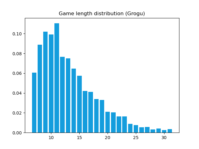
If you play against Grogu, you will soon notice that the estimated Q-values drop and are actually very bad estimates: this might come from the fact that the number of moves against the dumb opponent is very limited. Here is a barplot of the estimated distribution of the length of the games between Grogu and his opponent:
Yoda
Playing with Grogu is fun for a while but I still wanted to try and make an AI a little bit more capable. I therefore trained a DDQN with the following architecture:
- First layer of size 42
- Second layer of size 180
- Third layer of size 180
- Fourth layer of size 180
- Output layer of size 7
- The dumb opponent that met Grogu (looks for an easy win and plays randomly if he can't find one).
- A slightly smarter one that will also block a winning move if there is one for Yoda.